1.  Introduction

Diffusion Denoising Probabilistic Models (DDPM) have emerged as a powerful class of generative models in machine learning. They have shown remarkable capabilities in generating high-quality images, audio, and other data types. In this guide, we will derive the fundamental concepts behind DDPMs, explain their mathematical foundations, and provide insights into their implementation.

2.  Prior Knowledge

2.1.  Probabilistic Notations

Before diving into DDPMs, let’s clarify some probabilistic notations that will be used throughout this guide:

• $p(x)$: Probability density function (PDF) of a random variable $x$.

If we want to calculate the probability that $x$ falls within a specific range, we integrate $p(x)$ over that range.

$$P(a \leq x \leq b) = \int_{a}^{b} p(x) \, \mathrm{d}x$$

where $P$ is the probability measure.

• $p(x|y)$: Conditional probability density function of $x$ given $y$.

$$p(x|y) = \frac{p(x, y)}{p(y)}$$

• $\mathbb{E}[f(x)]$: Expectation of random variable $f(x)$.

$$\mathbb{E}[f(x)] = \int p(x) f(x) \, \mathrm dx$$

• $\mathbb{E}_{p}[f(x)]$: Expectation of function $f(x)$ with respect to the distribution $p(x)$.

$$\mathbb{E}_{q}[f(x)] = \int q(x) f(x) \, \mathrm dx$$

• $p(x)=\mathcal{N}(x;\mu, \sigma^2)$ indicates that $X\sim p(x)$ follows a Gaussian distribution with mean $\mu$ and variance $\sigma^2$. The variable before the semicolon is the random variable, and the variables after the semicolon are the parameters of the distribution.

2.2.  Bayes’ Theorem

Bayes’ theorem is a fundamental concept in probability theory that relates conditional probabilities. It states that:

$$p(x|y) = \frac{p(y|x)p(x)}{p(y)}$$

If we center our attention on $x$, we can interpret Bayes’ theorem as follows:

• $p(x|y)$ is the posterior probability of $x$ given $y$, which represents our updated belief about $x$ after observing $y$.
• $p(y|x)$ is the likelihood of observing $y$ given $x$, which indicates how probable the observation $y$ is for a specific value of $x$.
• $p(x)$ is the prior probability of $x$, which represents our initial belief about $x$ before observing $y$.
• $p(y)$ is the marginal likelihood of $y$, which serves as a normalizing constant to ensure that the posterior probability sums to 1.

Example:

Suppose there is a rare disease that affects 1% of the population. A diagnostic test for this disease has a 99% accuracy rate, which means if someone has the disease, the test will correctly identify them as positive 99% of the time. While, if someone does not have the disease, the test will incorrectly identify them as positive 2% of the time, calling it a false positive. If a person tests positive, what is the probability that they actually have the disease?
Let $D$ be the event that the person has the disease, and $T$ be the event that the test result is positive. We want to find $p(D|T)$.
Let’s define the known probabilities:

• $p(D) = 0.01$ (prior probability of having the disease)
• $p(\neg D) = 0.99$ (prior probability of not having the disease)
• $p(T|D) = 0.99$ (likelihood of testing positive given the disease)
• $p(T|\neg D) = 0.02$ (likelihood of testing positive given no disease)
  Using Bayes’ theorem, we can calculate the posterior probability $p(D|T)$:

$$p(D|T) = \frac{p(T|D)p(D)}{p(T)}$$

To find $p(T)$, we can use the law of total probability:

$$p(T) = p(T|D)p(D) + p(T|\neg D)p(\neg D)$$

this gives us the total probability of testing positive, considering both cases (having the disease and testing positive, not having the disease and testing positive).

Now we can plug in the values:

$$p(T) = (0.99)(0.01) + (0.02)(0.99) = 0.0099 + 0.0198 = 0.0297$$

Now we can calculate $p(D|T)$:

$$p(D|T) = \frac{(0.99)(0.01)}{0.0297} = \frac{0.0099}{0.0297} \approx 0.3333$$

Therefore, if a person tests positive, there is approximately a 33.33% chance that they actually have the disease, despite the high accuracy of the test. This counterintuitive result highlights the importance of considering prior probabilities when interpreting test results.

2.3.  Additive Property of Gaussian Distribution

The Gaussian (or normal) distribution is a continuous probability distribution characterized by its mean $\mu$ and variance $\sigma^2$. A key property of Gaussian distributions is that the sum of two independent Gaussian random variables is also a Gaussian random variable. Specifically, if we have two independent Gaussian random variables:

$$\begin{aligned} X_1 \sim \mathcal{N}(\mu_1, \sigma_1^2)\\ X_2 \sim \mathcal{N}(\mu_2, \sigma_2^2) \end{aligned}$$

Then, their sum $Y = X_1 + X_2$ is also Gaussian distributed:

$$Y \sim \mathcal{N}(\mu_1 + \mu_2, \sigma_1^2 + \sigma_2^2)$$

if $Y = X_1 - X_2$, then:

$$Y \sim \mathcal{N}(\mu_1 - \mu_2, \sigma_1^2 + \sigma_2^2)$$

We can extend this property to any linear combination of independent Gaussian random variables. For example, if we have:

$$Y = aX_1 + bX_2 + c$$

where $a$, $b$, and $c$ are constants, then $Y$ is also Gaussian distributed:

$$Y \sim \mathcal{N}(a\mu_1 + b\mu_2 + c, a^2\sigma_1^2 + b^2\sigma_2^2)$$

2.4.  Kullback-Leibler (KL) Divergence

Kullback-Leibler (KL) divergence is a measure of how one probability distribution diverges from a second, expected probability distribution. It is often used in creating a loss function for training probabilistic models, if we want to train a model to approximate a target distribution $p(x)$ with a model distribution $q(x)$, we can minimize the KL divergence from $p$ to $q$:

$$D_{KL}(p || q) = \int p(x) \log \frac{p(x)}{q(x)} \, \mathrm{dx} = \mathbb{E}_{p} \left[ \log \frac{p(x)}{q(x)} \right]$$

The KL divergence of Gaussian distributions has a closed-form solution. If we have two Gaussian distributions:

$$\begin{aligned} p(x) = \mathcal{N}(\mu_p, \Sigma_p^2)\\ q(x) = \mathcal{N}(\mu_q, \Sigma_q^2) \end{aligned}$$

$$\begin{aligned} p(x) = \frac{1}{(2\pi)^{k/2} |\Sigma_p|^{1/2}} \exp\left(-\frac{1}{2}(x - \mu_p)^T \Sigma_p^{-1} (x - \mu_p)\right) \\ q(x) = \frac{1}{(2\pi)^{k/2} |\Sigma_q|^{1/2}} \exp\left(-\frac{1}{2}(x - \mu_q)^T \Sigma_q^{-1} (x - \mu_q)\right) \end{aligned}$$

where $|\cdot|$ denotes the determinant of a matrix, we plug these PDFs into the KL divergence formula and simplify to get:

$$D_{KL}(p || q) = \mathbb{E}_{p} \left[ \log \frac{p(x)}{q(x)} \right]$$

with three parts:

Part 1:

$$\frac{1}{2} \left(\log |\Sigma_q| - \log |\Sigma_p|\right)$$

Part 2:

$$\frac{1}{2} \mathbb{E}_{p} \left[ (x - \mu_q)^T \Sigma_q^{-1} (x - \mu_q) \right]$$

Since $(x-\mu_p)^T \Sigma_p^{-1} (x-\mu_p)$ is actually a scalar, for a scalar, its trace is itself. Therefore, we can rewrite Part 2 as:

$$\frac{1}{2} \mathbb{E}_{p} \left[ \text{tr}\left((x - \mu_p)^T \Sigma_p^{-1} (x - \mu_p)\right) \right]$$

Using the cyclic property of the trace operator $\text{tr}(ABC) = \text{tr}(CAB) = \text{tr}(BCA)$, we can further simplify it to:

$$\begin{aligned} &\frac{1}{2} \mathbb{E}_{p} \left[ \text{tr}\left(\Sigma_p^{-1} (x - \mu_p)(x - \mu_p)^T\right) \right]\\ =& \frac{1}{2} \text{tr}\left(\Sigma_p^{-1} \mathbb{E}_{p} \left[ (x - \mu_p)(x - \mu_p)^T \right] \right)\\ =& \frac{1}{2} \text{tr}\left(\Sigma_p^{-1} \Sigma_p \right) = \frac{1}{2} \text{tr}(I) = \frac{k}{2} \end{aligned}$$

Part 3:

$$\begin{aligned} &\frac{1}{2} \mathbb{E}_{p} \left[ (x-\mu_p + \mu_p - \mu_q)^T \Sigma_q^{-1} (x-\mu_p + \mu_p - \mu_q) \right] \\ =& \frac{1}{2} \mathbb{E}_{p} \left[\text{tr}\left((x-\mu_p + \mu_p - \mu_q)^T \Sigma_q^{-1} (x-\mu_p + \mu_p - \mu_q)\right) \right] \\ =& \frac{1}{2} \mathbb{E}_{p} \left[\text{tr}\left(\Sigma_q^{-1} (x-\mu_p + \mu_p - \mu_q)(x-\mu_p + \mu_p - \mu_q)^T\right) \right] \\ =& \frac{1}{2} \text{tr}\left(\Sigma_q^{-1} \mathbb{E}_{p} \left[ (x-\mu_p + \mu_p - \mu_q)(x-\mu_p + \mu_p - \mu_q)^T \right] \right) \\ =& \mathbb{E}_{p}\!\left[(x-\mu_p)(x-\mu_p)^T\right] + (\mu_p-\mu_q)(\mu_p-\mu_q)^T + \underbrace{\mathbb{E}_{p}\!\left[(x-\mu_p)(\mu_p-\mu_q)^T\right]}_{=\,0} + \underbrace{\mathbb{E}_{p}\!\left[(\mu_p-\mu_q)(x-\mu_p)^T\right]}_{=\,0}\\ =& \frac{1}{2} \text{tr}\left(\Sigma_q^{-1} \mathbb{E}_{p} \left[ (x-\mu_p)(x-\mu_p)^T + (\mu_p - \mu_q)(\mu_p - \mu_q)^T \right] \right) \\ =& \frac{1}{2} \text{tr}\left(\Sigma_q^{-1} \Sigma_p\right) + \frac{1}{2} \text{tr}((\mu_p - \mu_q)^T \Sigma_q^{-1} (\mu_p - \mu_q))\\ =& \frac{1}{2} \text{tr}\left(\Sigma_q^{-1} \Sigma_p\right) + \frac{1}{2} (\mu_p - \mu_q)\Sigma_q^{-1}(\mu_p - \mu_q)^T \\ \end{aligned}$$

Combining all three parts, we obtain the closed-form expression for the KL divergence between two Gaussian distributions:

$$D_{KL}(p || q) = \frac{1}{2} \left(\log |\Sigma_q| - \log |\Sigma_p|\right) + \frac{k}{2} + \frac{1}{2} \text{tr}\left(\Sigma_q^{-1} \Sigma_p\right) + \frac{1}{2} (\mu_p - \mu_q)\Sigma_q^{-1}(\mu_p - \mu_q)^T$$

3.  The Big Picture

The goal of DDPM is to learn a generative model that can produce samples from a target data distribution $p_{\text{data}}(z)$. Here we need to define what is “data” and what is “generation”.

“Data” refers to the real-world samples we want our model to learn from, such as images, audio, or text. These samples are drawn from an unknown distribution $p_{\text{data}}(z)$ that we aim to approximate. What we have access to are finite samples $z_1, z_2, \ldots, z_N$ from this distribution, which we use to train our model.

“Generation” refers to the process of creating plausible new samples $z_{\text{new}}$ from the learned model. I use the term “plausible” because the generated samples should resemble the real data in terms of structure and characteristics, but they do not need to be exact replicas of any specific training sample. The goal is to capture the underlying distribution of the data so that the model can produce diverse and realistic samples. In the term of mathematics, we want to learn a model distribution $p_{\theta}(z)$ that approximates the true data distribution $p_{\text{data}}(z)$, and we can generate new samples $z_{\text{new}}$ by sampling from $p_{\theta}(z)$, which makes $p_{\text{data}}(z_{\text{new}})$ not too small.

4.  Overview of Diffusion Denoising Probabilistic Models (DDPM)

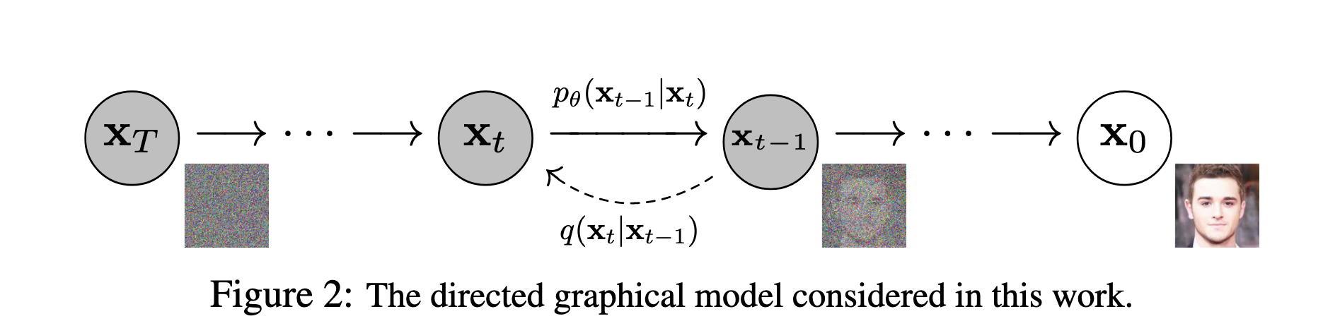
The core idea of DDPM is to model the data generation process as a gradual denoising of a noisy input. The model consists of two main processes: the forward diffusion process and the reverse denoising process.

What the model actually learns is the reverse denoising process, which starts from pure noise and iteratively denoises it to produce a clean sample that resembles the training data. This process is parameterized by a neural network that predicts the noise component at each step, allowing the model to gradually refine the noisy input into a high-quality output.

4.1.  Reverse Denoising Process

Let’s denote the clean data sample as $\mathrm x_0$ and the noisy sample at step $t$ as $\mathrm x_t$. At the final step $T$, $\mathrm x_T$ is essentially pure noise $p(\mathrm x_T) = \mathcal{N}(\mathrm x_T;\mathbf 0, \mathbf I)$.

$$p_\theta(\mathrm x_{0:T}) := p(\mathrm x_T) \prod_{t=1}^{T} p_\theta(\mathrm x_{t-1}|\mathrm x_t)$$

where $\mathrm x_{0:T}$ denotes the sequence of all latent variables from the initial clean sample to the final noisy sample. This formulation captures the entire generative process, starting from pure noise $\mathrm x_T$ and progressively denoising it to obtain the clean sample $\mathrm x_0$, using a markovian structure where each step depends only on the previous one.

If we fixed a $\mathrm x_0$, there may be infinite possible $\mathrm x_{1:T}$ that can lead to this $\mathrm x_0$. Therefore, to get the probability of generating $\mathrm x_0$, we need to marginalize out all possible $\mathrm x_{1:T}$:

$$p_\theta(\mathrm x_0) = \int p_\theta(\mathrm x_{0:T}) \, \mathrm d \mathrm x_{1:T}$$

For each denoising step, we model the conditional probability $p_\theta(\mathrm x_{t-1}|\mathrm x_t)$ as a Gaussian distribution:

$$p_\theta(\mathrm x_{t-1}|\mathrm x_t) = \mathcal{N}(\mathrm x_{t-1}; \mu_\theta(\mathrm x_t, t), \Sigma_\theta(\mathrm x_t, t))$$

where $\mu_\theta(\mathrm x_t, t)$ and $\Sigma_\theta(\mathrm x_t, t)$ are the mean and covariance predicted by a neural network parameterized by $\theta$ at step $t$.

4.2.  Forward Diffusion Process

The forward diffusion process gradually adds noise to the clean data sample $\mathrm x_0$ over $T$ steps, resulting in a sequence of noisy samples $\mathrm x_1, \mathrm x_2, \ldots, \mathrm x_T$. This process is defined as:

$$q(\mathrm x_{1:T}|\mathrm x_0) := \prod_{t=1}^{T} q(\mathrm x_t|\mathrm x_{t-1})$$

where each step adds Gaussian noise to the previous sample:

$$q(\mathrm x_t|\mathrm x_{t-1}) = \mathcal{N}(\mathrm x_t; \sqrt{1 - \beta_t} \mathrm x_{t-1}, \beta_t \mathbf I)$$

Here, $\beta_t$ is a variance schedule that controls the amount of noise added at each step. As $t$ increases, more noise is added, and by the final step $T$, the sample $\mathrm x_T$ becomes nearly indistinguishable from pure Gaussian noise.

However, for training purposes, we don’t want to sample $\mathrm x_t$ sequentially from $\mathrm x_0$ to $\mathrm x_T$, this cost too much time. Fortunately, due to the properties of Gaussian distributions, we can directly sample $\mathrm x_t$ from $\mathrm x_0$ without going through all intermediate steps.

Proof:

Since each step in the forward diffusion process is Gaussian, the composition of these Gaussian steps results in another Gaussian distribution. As Fomula (29) shows, we can derive the mean and variance of $q(\mathrm x_t|\mathrm x_0)$ by recursively applying the properties of Gaussian distributions:

$$\mathrm x_t = \sqrt{1 - \beta_t} \mathrm x_{t-1} + \sqrt{\beta_t} \epsilon_{t-1}, \quad \epsilon_{t-1} \sim \mathcal{N}(\mathbf 0, \mathbf I)$$

where $\sqrt{1 - \beta_t} \mathrm x_{t-1}$ contribute to the mean, and $\sqrt{\beta_t} \epsilon_{t-1}$ contribute to the variance.

$$\mathrm x_t = \sqrt{\bar \alpha_t} \mathrm x_0 + \sqrt{1 - \bar \alpha_t} \epsilon, \quad \epsilon \sim \mathcal{N}(\mathbf 0, \mathbf I)$$

By recursively substituting $\mathrm x_{t-1}$ back to $\mathrm x_0$, we can express $\mathrm x_t$ directly in terms of $\mathrm x_0$ and the accumulated noise:

$$\begin{aligned} \mathrm x_t &= \sqrt{1 - \beta_t} \left( \sqrt{1 - \beta_{t-1}} \mathrm x_{t-2} + \sqrt{\beta_{t-1}} \epsilon_{t-2} \right) + \sqrt{\beta_t} \epsilon_{t-1} \\ &= \sqrt{(1 - \beta_t)(1 - \beta_{t-1})} \mathrm x_{t-2} + \sqrt{(1 - \beta_t)\beta_{t-1}} \epsilon_{t-2} + \sqrt{\beta_t} \epsilon_{t-1} \\ &\vdots \\ &= \sqrt{\prod_{s=1}^{t} (1 - \beta_s)} \mathrm x_0 + \sum_{s=1}^{t} \sqrt{\beta_s \prod_{u=s+1}^{t} (1 - \beta_u)} \epsilon_{s-1}\\ &\sim \mathcal{N}\left(\sqrt{\bar \alpha_t} \mathrm x_0, \left(1 - \bar \alpha_t\right) \mathbf I\right) \end{aligned}$$

where $\alpha_t = 1 - \beta_t$ and $\bar \alpha_t = \prod_{s=1}^{t} \alpha_s$.

So, we have:

$$q(\mathrm x_t|\mathrm x_0) = \mathcal{N}(\mathrm x_t; \sqrt{\bar \alpha_t} \mathrm x_0, (1 - \bar \alpha_t) \mathbf I)$$

4.3.  Loss Function

To train the DDPM, we need to define a loss function that measures how well the model’s predicted denoising matches the true denoising process. We can use the variational lower bound (VLB) on the negative log-likelihood of the data as our loss function:

$$\begin{aligned} \mathbb E[-\log p_\theta(\mathrm x_0)] &= \mathbb E[-\log \int p_\theta(\mathrm x_{0:T}) \, \mathrm d \mathrm x_{1:T}] \\ &= \mathbb E\left[-\log \int q(\mathrm x_{1:T}|\mathrm x_0) \frac{p_\theta(\mathrm x_{0:T})}{q(\mathrm x_{1:T}|\mathrm x_0)} \, \mathrm d \mathrm x_{1:T}\right] \\ &= \mathbb E\left[-\log \mathbb E_{q} \left[\frac{p_\theta(\mathrm x_{0:T})}{q(\mathrm x_{1:T}|\mathrm x_0)}\right]\right] \\ &= -\log \mathbb E_q \left[ \frac{q(\mathrm x_{1:T}|\mathrm x_0)}{p_\theta(\mathrm x_{0:T})}\right] \\ \end{aligned}$$

Because $\log$ is a concave function, we can apply Jensen’s inequality to obtain the variational lower bound:

$$\begin{aligned} \mathbb E_q[-\log p_\theta(\mathrm x_0)] &\leq \mathbb E_q\left[-\log \frac{p_\theta(\mathrm x_{0:T})}{q(\mathrm x_{1:T}|\mathrm x_0)}\right] := \mathcal{L}(\theta)\\ \end{aligned}$$

However, this expression is still intractable due to the integral over all possible $\mathrm x_{1:T}$. To make it tractable, we can decompose the loss into a sum of KL divergences at each time step:

$$\begin{aligned} \mathcal{L}(\theta) &= \mathbb E_q\left[-\log p(\mathrm x_T) - \sum_{t\geq 1} \log p_\theta(\mathrm x_{t-1}|\mathrm x_t) + \sum_{t\geq 1} \log q(\mathrm x_t|\mathrm x_{t-1})\right] \\ &= \mathbb E_q\left[-\log p(\mathrm x_T) - \sum_{t>1} \log \frac{p_\theta(\mathrm x_{t-1}|\mathrm x_t)}{q(\mathrm x_t|\mathrm x_{t-1})} - \log \frac{p_\theta(\mathrm x_0|\mathrm x_1)}{q(\mathrm x_1|\mathrm x_0)}\right] \\ \end{aligned}$$

Then, we use the Bayes’ theorem to rewrite the $q(\mathrm x_t|\mathrm x_{t-1})$ term:

$$q(\mathrm x_t|\mathrm x_{t-1}) = \frac{q(\mathrm x_{t-1}|\mathrm x_t,\mathrm x_0) q(\mathrm x_t|\mathrm x_0)}{q(\mathrm x_{t-1}|\mathrm x_0)}$$

This gives us:

$$\begin{aligned} &\mathcal{L}(\theta) = \mathbb E_q\left[-\log p(\mathrm x_T) - \sum_{t>1} \log \frac{p_\theta(\mathrm x_{t-1}|\mathrm x_t) q(\mathrm x_{t-1}|\mathrm x_0)}{q(\mathrm x_{t-1}|\mathrm x_t,\mathrm x_0) q(\mathrm x_t|\mathrm x_0)} - \log \frac{p_\theta(\mathrm x_0|\mathrm x_1)}{q(\mathrm x_1|\mathrm x_0)}\right] \\ \end{aligned}$$

Rearranging the terms, we can cancel out $q(\mathrm x_{t-1}|\mathrm x_0)$ and $q(\mathrm x_t|\mathrm x_0)$ in the summation:

$$\begin{aligned} \sum_{t>1} \log \frac{q(\mathrm x_{t-1}|\mathrm x_0)}{ q(\mathrm x_t|\mathrm x_0)}&=\log q(\mathrm x_1|\mathrm x_0) - \log q(\mathrm x_2|\mathrm x_0) + \log q(\mathrm x_2|\mathrm x_0) - \log q(\mathrm x_3|\mathrm x_0) + \ldots+ \log q(\mathrm x_{T-1}|\mathrm x_0) - \log q(\mathrm x_T|\mathrm x_0)\\ &=\log q(\mathrm x_1|\mathrm x_0) - \log q(\mathrm x_T|\mathrm x_0) \end{aligned}$$

So the loss function becomes:

$$\begin{aligned} \mathcal{L}(\theta)&= \mathbb E_q\left[-\log p(\mathrm x_T) + \sum_{t>1} \log \frac{q(\mathrm x_{t-1}|\mathrm x_t,\mathrm x_0)}{p_\theta(\mathrm x_{t-1}|\mathrm x_t)} + \log q(\mathrm x_T|\mathrm x_0) - \log p_\theta(\mathrm x_0|\mathrm x_1) + \log q(\mathrm x_1|\mathrm x_0)\right] \\ &= \mathbb E_q\left[-\log \frac{p(\mathrm x_T)}{q(\mathrm x_T|\mathrm x_0)} - \sum_{t>1} \log \frac{p_\theta(\mathrm x_{t-1}|\mathrm x_t)}{q(\mathrm x_{t-1}|\mathrm x_t,\mathrm x_0)} - \log \frac{p_\theta(\mathrm x_0|\mathrm x_1)}{q(\mathrm x_1|\mathrm x_0)}\right] \\ &= \mathbb E_q\left[D_{KL}(q(\mathrm x_T|\mathrm x_0) || p(\mathrm x_T)) + \sum_{t>1} D_{KL}(q(\mathrm x_{t-1}|\mathrm x_t,\mathrm x_0) || p_\theta(\mathrm x_{t-1}|\mathrm x_t)) + D_{KL}(q(\mathrm x_1|\mathrm x_0) || p_\theta(\mathrm x_0|\mathrm x_1))\right] \\ \end{aligned}$$

Now, we have decomposed the loss function into three main components:

$$\mathcal{L}(\theta)=\mathbb E_q\!\Big[ \underbrace{D_{KL}(q(\mathrm x_T|\mathrm x_0) \,||\, p(\mathrm x_T))}_{\mathcal L_T} + \underbrace{\sum_{t>1} D_{KL}(q(\mathrm x_{t-1}|\mathrm x_t,\mathrm x_0) \,||\, p_\theta(\mathrm x_{t-1}|\mathrm x_t))}_{\mathcal L_{t-1}} + \underbrace{D_{KL}(q(\mathrm x_1|\mathrm x_0) \,||\, p_\theta(\mathrm x_0|\mathrm x_1))}_{\mathcal L_0} \Big]$$

Since each term in the loss function is a KL divergence between two Gaussian distributions, we can use the closed-form solution of KL divergence for Gaussian distributions to compute the loss efficiently during training. This allows us to optimize the model parameters $\theta$ using gradient descent, ultimately enabling the DDPM to learn to generate high-quality samples from the target data distribution.

• For $\mathcal L_T$:
  Since DDPM fixed the $\beta_t$ schedule, so $\mathcal{L}_T$ is not relevant to the optimization, we can ignore it during training.

• For $\mathcal L_{t-1}$:
  To compute $\mathcal{L}_{t-1}$, we need to determine the posterior distribution $q(\mathrm x_{t-1}|\mathrm x_t,\mathrm x_0)$. Using Bayes’ theorem, we have:

$$q(\mathrm x_{t-1}|\mathrm x_t,\mathrm x_0) = \frac{q(\mathrm x_t|\mathrm x_{t-1}, \mathrm x_0) q(\mathrm x_{t-1}|\mathrm x_0)}{q(\mathrm x_t|\mathrm x_0)}$$

Since the forward process is Markovian, we know that $q(\mathrm x_t|\mathrm x_{t-1}, \mathrm x_0) = q(\mathrm x_t|\mathrm x_{t-1})$. Therefore, we can rewrite the equation as:

$$q(\mathrm x_{t-1}|\mathrm x_t,\mathrm x_0) = \frac{q(\mathrm x_t|\mathrm x_{t-1}) q(\mathrm x_{t-1}|\mathrm x_0)}{q(\mathrm x_t|\mathrm x_0)}$$

Combining with Formula (37), (33), we directly plug in the distributions parameters into the PDF of Gaussian distribution:

$$\begin{aligned} q(\mathrm x_{t-1}|\mathrm x_t,\mathrm x_0) &= \frac{1}{(2\pi)^{d/2} |\beta_t \mathbf I|^{1/2}} \exp\left(-\frac{1}{2}(\mathrm x_t - \sqrt{1 - \beta_t} \mathrm x_{t-1})^T (\beta_t \mathbf I)^{-1} (\mathrm x_t - \sqrt{1 - \beta_t} \mathrm x_{t-1})\right) \\ &\quad \cdot \frac{1}{(2\pi)^{d/2} |(1 - \bar \alpha_{t-1}) \mathbf I|^{1/2}} \exp\left(-\frac{1}{2}(\mathrm x_{t-1} - \sqrt{\bar \alpha_{t-1}} \mathrm x_0)^T ((1 - \bar \alpha_{t-1}) \mathbf I)^{-1} (\mathrm x_{t-1} - \sqrt{\bar \alpha_{t- 1}} \mathrm x_0)\right) \\ &\quad \cdot \frac{(2\pi)^{d/2} |(1 - \bar \alpha_t) \mathbf I|^{1/2}}{\exp\left(-\frac{1}{2}(\mathrm x_t - \sqrt{\bar \alpha_t} \mathrm x_0)^T ((1 - \bar \alpha_t) \mathbf I)^{-1} (\mathrm x_t - \sqrt{\bar \alpha_t} \mathrm x_0)\right)} \\ &\ldots \end{aligned}$$

After simplifying the expression, we find that the posterior distribution $q(\mathrm x_{t-1}|\mathrm x_t,\mathrm x_0)$ is also a Gaussian distribution:

$$q(\mathrm x_{t-1}|\mathrm x_t,\mathrm x_0) = \mathcal{N}(\mathrm x_{t-1}; \tilde \mu_t(\mathrm x_t, \mathrm x_0), \tilde \beta_t \mathbf I)$$

where

$$\tilde \mu_t(\mathrm x_t, \mathrm x_0) = \frac{\sqrt{\bar \alpha_{t-1}} \beta_t}{1 - \bar \alpha_t} \mathrm x_0 + \frac{\sqrt{\alpha_t} (1 - \bar \alpha_{t-1})}{1 - \bar \alpha_t} \mathrm x_t$$

and

$$\tilde \beta_t = \frac{1 - \bar \alpha_{t-1}}{1 - \bar \alpha_t} \beta_t$$

Now, we can compute the KL divergence $\mathcal{L}_{t-1}$ between the posterior distribution $q(\mathrm x_{t-1}|\mathrm x_t,\mathrm x_0)$ and the model’s predicted distribution $p_\theta(\mathrm x_{t-1}|\mathrm x_t)$ using the closed-form solution for KL divergence between two Gaussian distributions:

$$\begin{aligned} \mathcal{L}_{t-1} &= \mathbb{E}_q\Big [D_{KL}(q(\mathrm x_{t-1}|\mathrm x_t,\mathrm x_0) || p_\theta(\mathrm x_{t-1}|\mathrm x_t)) \Big]\\ &= \mathbb{E}_q\Big[\frac{1}{2} \left(\log |\Sigma_\theta(\mathrm x_t, t)| - \log |\tilde \beta_t \mathbf I|\right) + \frac{d}{2} + \frac{1}{2} \text{tr}\left(\Sigma_\theta(\mathrm x_t, t)^{-1} \tilde \beta_t \mathbf I\right) + \frac{1}{2} (\tilde \mu_t(\mathrm x_t, \mathrm x_0)\\ &\quad- \mu_\theta(\mathrm x_t, t))^T \Sigma_\theta(\mathrm x_t, t)^{-1} (\tilde \mu_t(\mathrm x_t, \mathrm x_0) - \mu_\theta(\mathrm x_t, t)) \Big]\\ \end{aligned}$$

DDPM made a simplification by fixing the covariance $\Sigma_\theta(\mathrm x_t, t)$ to $\sigma_t^2 \mathbf I$, which allows us to ignore the first three terms during optimization because they do not depend on the model parameters $\theta$. Therefore, the loss term $\mathcal{L}_{t-1}$ simplifies to:

$$\begin{aligned} \mathcal{L}_{t-1} &= \mathbb{E}_q\Big[\frac{1}{2} (\tilde \mu_t(\mathrm x_t, \mathrm x_0) - \mu_\theta(\mathrm x_t, t))^T \Sigma_\theta(\mathrm x_t, t)^{-1} (\tilde \mu_t(\mathrm x_t, \mathrm x_0) - \mu_\theta(\mathrm x_t, t)) + \text{C}\Big]\\ &=\mathbb{E}_q\Big[\frac{1}{2} (\tilde \mu_t(\mathrm x_t, \mathrm x_0) - \mu_\theta(\mathrm x_t, t))^T \frac{1}{\sigma_t^2} \mathbf I (\tilde \mu_t(\mathrm x_t, \mathrm x_0) - \mu_\theta(\mathrm x_t, t)) + \text{C}\Big]\\ &= \mathbb{E}_q\Big[\frac{1}{2 \sigma_t^2} \|\tilde \mu_t(\mathrm x_t, \mathrm x_0) - \mu_\theta(\mathrm x_t, t)\|^2 + \text{C}\Big] \end{aligned}$$

Applied Fomula (33), we can express $\mathrm x_t$ in terms of $\mathrm x_0$ and the noise component $\epsilon\sim \mathcal{N}(0, \mathbf I)$:

$$\mathrm x_t(\mathrm x_0, \epsilon) = \sqrt{\bar \alpha_t} \mathrm x_0 + \sqrt{1 - \bar \alpha_t} \epsilon$$

Then we plug this into the loss function, using Formula (46):

$$\begin{aligned} \mathcal{L}_{t-1} - \text{C} &= \mathbb{E}_{\mathrm x_0, \epsilon}\Big[\frac{1}{2 \sigma_t^2} \big\|\tilde \mu_t(\mathrm x_t(\mathrm x_0, \epsilon), \frac{1}{\sqrt{\bar \alpha_t}}(\mathrm x_t(\mathrm x_0, \epsilon) - \sqrt{1 - \bar \alpha_t} \epsilon)) - \mu_\theta(\mathrm x_t(\mathrm x_0, \epsilon), t)\big\|^2\Big]\\ &= \mathbb{E}_{\mathrm x_0, \epsilon}\Bigg[\frac{1}{2 \sigma_t^2} \Big\|\frac{\sqrt{\bar \alpha_{t-1}} \beta_t}{1 - \bar \alpha_t} \frac{1}{\sqrt{\bar \alpha_t}}(\mathrm x_t(\mathrm x_0, \epsilon) - \sqrt{1 - \bar \alpha_t} \epsilon) + \frac{\sqrt{\alpha_t} (1 - \bar \alpha_{t-1})}{1 - \bar \alpha_t} \mathrm x_t(\mathrm x_0, \epsilon) - \mu_\theta(\mathrm x_t(\mathrm x_0, \epsilon), t)\Big\|^2\Bigg]\\ &= \mathbb{E}_{\mathrm x_0, \epsilon}\Bigg[\frac{1}{2 \sigma_t^2} \Big\|\frac{1}{\sqrt{\bar \alpha_t}} \big(\mathrm x_t(\mathrm x_0,\epsilon) - \frac{\beta_t}{\sqrt{1-\bar \alpha_t}}\epsilon\big) - \mu_\theta(\mathrm x_t(\mathrm x_0, \epsilon), t)\Big\|^2\Bigg]\\ \end{aligned}$$

Here we changed the expectation from $q$ to $\mathrm x_0$ and $\epsilon$, because currently $\mathrm x_t$ is fully determined by $\mathrm x_0$ and $\epsilon$.

Previously, the $q$ of $\mathbb E_q$ means for all $\mathrm x_{1:T}$ follow $q(\mathrm x_{1:T}|\mathrm x_0)$, but now we only need to sample $\mathrm x_0$ from the data distribution and $\epsilon$ from the standard normal distribution to compute $\mathrm x_t$. This significantly simplifies the training process, as we no longer need to sample the entire sequence of noisy samples $\mathrm x_{1:T}$.

With the Formula (51), out training goal becomes:

$$\mu_\theta(\mathrm x_t, t) \approx \frac{1}{\sqrt{\bar \alpha_t}} \left(\mathrm x_t - \frac{\beta_t}{\sqrt{1 - \bar \alpha_t}} \epsilon\right)$$

then we can reparameterize the neural network to predict the noise component $\epsilon_\theta(\mathrm x_t, t)$ instead of the mean $\mu_\theta(\mathrm x_t, t)$:

$$\mu_\theta(\mathrm x_t, t) = \frac{1}{\sqrt{\bar \alpha_t}} \left(\mathrm x_t - \frac{\beta_t}{\sqrt{1 - \bar \alpha_t}} \epsilon_\theta(\mathrm x_t, t)\right)$$

Now, $\epsilon_\theta$ becomes a function approximator that learns to predict the noise $\epsilon$ added at each step of the diffusion process from the noisy sample $\mathrm x_t$.

Because we defined $p_\theta(\mathrm x_{t-1}|\mathrm x_t)$ as a Gaussian distribution $\mathcal{N}(\mathrm x_{t-1}; \mu_\theta(\mathrm x_t, t), \Sigma_\theta(\mathrm x_t, t))$ in Formula (27), where a made an assumption that the covariance $\Sigma_\theta(\mathrm x_t, t) = \sigma_t^2 \mathbf I$ is fixed. Therefore, we can now express the mean $\mu_\theta$ in terms of the predicted noise $\epsilon_\theta$:

$$\begin{aligned} \mathrm x_{t-1}&=\mu_\theta(\mathrm x_t, t) + \sigma_t \mathbf z, \quad \mathbf z \sim \mathcal{N}(\mathbf 0, \mathbf I) \\ &= \frac{1}{\sqrt{\bar \alpha_t}} \left(\mathrm x_t - \frac{\beta_t}{\sqrt{1 - \bar \alpha_t}} \epsilon_\theta(\mathrm x_t, t)\right) + \sigma_t \mathbf z \end{aligned}$$

With the parameterization of $\epsilon_\theta$, we can now rewrite the Formula (51) loss function in terms of the predicted noise:

$$\begin{aligned} \mathcal{L}_{t-1} - \text{C} &= \mathbb{E}_{\mathrm x_0, \epsilon}\Bigg[\frac{1}{2 \sigma_t^2} \Big\|\frac{1}{\sqrt{\bar \alpha_t}} \big(\mathrm x_t(\mathrm x_0, \epsilon) - \frac{\beta_t}{\sqrt{1-\bar \alpha_t}}\epsilon\big) - \mu_\theta(\mathrm x_t(\mathrm x_0, \epsilon), t)\Big\|^2\Bigg]\\ &= \mathbb{E}_{\mathrm x_0, \epsilon}\Bigg[\frac{1}{2 \sigma_t^2} \Big\|\frac{1}{\sqrt{\bar \alpha_t}} \big(\mathrm x_t(\mathrm x_0, \epsilon) - \frac{\beta_t}{\sqrt{1-\bar \alpha_t}}\epsilon\big) - \frac{1}{\sqrt{\bar \alpha_t}} \left(\mathrm x_t(\mathrm x_0, \epsilon) - \frac{\beta_t}{\sqrt{1 - \bar \alpha_t}} \epsilon_\theta(\mathrm x_t(\mathrm x_0, \epsilon), t)\right)\Big\|^2\Bigg]\\ &= \mathbb{E}_{\mathrm x_0, \epsilon}\Bigg[\frac{\beta_t^2}{2 \sigma_t^2\alpha_t(1-\alpha_t)} \Big\|\epsilon - \epsilon_\theta(\mathrm x_t(\mathrm x_0, \epsilon), t)\Big\|^2\Bigg]\\ &= \mathbb{E}_{\mathrm x_0, \epsilon}\Bigg[\frac{\beta_t^2}{2 \sigma_t^2\alpha_t(1-\alpha_t)} \Big\|\epsilon - \epsilon_\theta(\sqrt{\bar \alpha_t}\mathrm x_0+\sqrt{1-\bar\alpha_t}\epsilon,t)\Big\|^2\Bigg]\\ \end{aligned}$$

Now, we have all we need to implement the training algorithm for DDPM.

\begin{algorithm}
\caption{Training}
\begin{algorithmic}
\REPEAT
    \STATE $\mathbf{x}_0 \sim q(\mathbf{x}_0)$
    \STATE $t \sim \text{Uniform}(\{1, \dots, T\})$
    \STATE $\boldsymbol{\epsilon} \sim \mathcal{N}(\mathbf{0}, \mathbf{I})$
    \STATE Take gradient descent step on
         $\nabla_{\boldsymbol{\theta}} \|\boldsymbol{\epsilon} - \boldsymbol{\epsilon}_{\boldsymbol{\theta}}(\sqrt{\bar{\alpha}_t}\mathbf{x}_0 + \sqrt{1 - \bar{\alpha}_t}\boldsymbol{\epsilon}, t)\|^2$
\UNTIL{converged}
\end{algorithmic}
\end{algorithm}

\begin{algorithm}
\caption{Sampling}
\begin{algorithmic}
\STATE $\mathbf{x}_T \sim \mathcal{N}(\mathbf{0}, \mathbf{I})$
\FOR{$t = T, \dots, 1$}
    \IF{$t > 1$}
        \STATE $\mathbf{z} \sim \mathcal{N}(\mathbf{0}, \mathbf{I})$
    \ELSE
        \STATE $\mathbf{z} = \mathbf{0}$
    \ENDIF
    \STATE $\mathbf{x}_{t-1} = \frac{1}{\sqrt{\alpha_t}}\left(\mathbf{x}_t - \frac{1-\alpha_t}{\sqrt{1-\bar{\alpha}_t}}\boldsymbol{\epsilon}_{\boldsymbol{\theta}}(\mathbf{x}_t, t)\right) + \sigma_t \mathbf{z}$
\ENDFOR
\RETURN $\mathbf{x}_0$
\end{algorithmic}
\end{algorithm}